Radiometric Identification Of Signals By Matched Whitening Transform Part 1
Apr 13, 2023
Abstract: Radiometric identification is the problem of attributing a signal to a specific source. In this work, a radiometric identification algorithm is developed using the whitening transformation. The approach stands out from the more established methods in that it works directly on the raw IQ data and hence is featureless. As such, the commonly used dimensionality reduction algorithms do not apply. The premise of the idea is that a data set is “most white” when projected on its whitening matrix than on any other. In practice, transformed data are never strictly white since the training and the test data differ. The Förstner-Moonen measure that quantifies the similarity of covariance matrices is used to establish the degree of whiteness. The whitening transform that produces a data set with the minimum Förstner-Moonen distance to a white noise process is the source signal. The source is determined by the output of the mode function operated on the Majority Vote Classifier decisions. Using the Förstner-Moonen measure presents a different perspective compared to maximum likelihood and Euclidean distance metrics. The whitening transform is also contrasted with the more recent deep-learning approaches that are still dependent on feature vectors with large dimensions and lengthy training phases. It is shown that the proposed method is simpler to implement, requires no feature vectors, needs minimal training and because of its non-iterative structure is faster than existing approaches.
According to relevant studies,cistanche is a common herb that is known as "the miracle herb that prolongs life". Its main component is cistanoside, which has various effects such as antioxidant, anti-inflammatory, and immune function promotion. The mechanism between cistanche and skin whitening lies in the antioxidant effect of cistanche glycosides. Melanin in human skin is produced by the oxidation of tyrosine catalyzed by tyrosinase, and the oxidation reaction requires the participation of oxygen, so the oxygen-free radicals in the body become an important factor affecting melanin production. Cistanche contains cistanoside, which is an antioxidant and can reduce the generation of free radicals in the body, thus inhibiting melanin production.

Click on How to Use Cistanche Tubulosa
For more info:
david.deng@wecistanche.com WhatApp:86 13632399501
1. Introduction
Radiometric identification is the problem of attributing a signal to the source; often brand or model. Source identification is accomplished by RF fingerprinting of devices by looking for signatures that may arise from manufacturing tolerances, imperfections, or normal statistical variations in production. There is considerable work in signal classification and modulation recognition [1,2]. However, radiometric identification does not neatly fit into either of the two categories. In many ways, radiometric identification is a more difficult problem as signals originating from different sources may have similar characteristics such as modulation, bit rates, pulse shapes, etc. This fact makes subtle device variations the main signature for radiometric identification. Such variations, however, are small, imperceptible, and difficult to model. Why radiometric identification is of interest are many folds. The military has been interested in this capability for some time as a means of identifying friendly from hostile radar [3,4]. Satellite communication may be faced with intentional or unintentional jamming from rogue sources. Knowing the source and the brand of the interferer may help identify the offending source. Radiometric identification is also a valuable tool in securing wireless devices. Spoofing attempts in wireless networks and IoT devices can be thwarted if the source of the signal could be identified and blocked [5,6]. It is more difficult to mimic device characteristics that are embedded in signals than to replicate modulation or pulse shaping.
Radiometric identification can be formulated in the context of a statistical classifier. The classical approach follows feature extraction and dimensionality reduction by techniques such as PCA and finally multiple discriminant analysis classifier [7,8]. In [9], Square Integral Bispectra (SIB) is used to extract the unique stray features of individual transmitted signals, followed by PCA to extract a low-dimensional feature vector. It has been observed that features retained after dimensionality reduction are not necessarily optimal for classification.

Combined optimization of dimensionality reduction and fingerprint classification is proposed in [10]. The idea is to drive dimensionality reduction by minimizing the classified- cation error and maximizing the mutual information between the reduced dimensionality features and the class label simultaneously. The RF fingerprint features are extracted from the statistics of the normalized instantaneous amplitude, phase, and frequency of the signal resulting in feature vectors with up to 960 dimensions. The dimensionality reduction problem remains, however. Feature extraction for transmitter identification algorithms has been developed to operate in either transient [11] or steady-state phases [12]. The transient phase is an analog state of the signal occurring right after the transmitter is activated whereas the steady state phase is characterized by modulation.
More recent work on radiometric identification has been influenced by the rise of deep learning (DL) tools. Examples are RF fingerprinting [13], IoT device fingerprinting [14], spectrum sensing [15], and RF device identification in cognitive networks [16]. What is still needed in all such work is the extraction of feature vectors followed by time-consuming dimensionality reduction. The feature vectors extracted in [10], for example, have 960 dimensions before dimensionality reduction. In other words, the main problem remains. The use of DL is often accomplished by the programming of off-the-shelf tools or the use of various convolutional neural networks (CNN) routines implemented in Matlab. For example, the compressed bispectrum is identified as the feature and then used to train a three-layer CNN [17]. What differs are the number of layers, taps, filters, activation functions, etc. Another example along this vein appears in [18] where Keras API is used with TensorFlow on the backend to distinguish distracted drivers. In [15], DL is implemented for RF device fingerprinting in the cognitive Zigbee networks using the time-domain complex baseband error signal as training and test data. The results show good accuracy (≈90%) but at high SNR (≥20 dB). In [19], the input data are preprocessed as Hilbert spectrum gray-scale images and achieve acceptable accuracy under moderate SNR levels (Avg 70% accuracy rate for SNR of 15 dB). A comprehensive performance comparison is shown for various DL algorithms in [13], reporting an average accuracy of 98% measured for 12 transmitters.
The fact that ML operates on much smaller data sets and requires much less training time compared to DL (hours of training [15]), provides more versatility to signal characteristics changes that occurs under different environmental circumstances (overheating, excess current, etc.), which can strongly affect the classification selected feature. This property of ML (data-driven) allows for fast feature updates and consequently results in higher accurate classification in the long term. In addition, the reduced complexity compared to DL allows for easier hardware implementation and fast on-the-fly classification.

Specific Emitter Identification (SEI) is another paradigm for radiometric identification [20–22]. The SEI approach attempts to identify the unique transmitter of a signal using only external feature measurements [22]. SEI is implemented in two stages, (1) transient signal state and (2) steady-state signal state. The transient approach applies to the particular signatures embedded in the signal as the transmitter powers up or down [23,24]. Transient approaches are more difficult to implement due to the unavailability or transient nature of the data that is often not accessible or saved. The steady-state approach refers to the period where transients have stabilized. The available features include modulation and preamble [25,26], among others. In modulation-based techniques, the received and the target constellations are compared where the difference creates an RF fingerprint [27]. A fast decision identification algorithm appears in [28]. Identification is based on the similarity of a signal vector and its comparison to patterns available in a database. The approach is classified as an example of SEI applied to radar identification. The algorithm was applied to hundreds of radar signal records that came from several different types of radars. In some cases, copies of the same type of radar were investigated. Weighing all features equally, an 85% correct recognition rate is reported for radar types. A mixed method of radar identification based on electromagnetic emission and intrapulse analysis appears in [29]. The premise is that electronic devices impart electrical features to the transmitted pulse. The signal model is N non-overlapping pushes from K transmitters. Linear Discriminant Analysis is used. Four distance metrics are used to classify the unknown pulse. It is reported that three copies of the same type of radar are successfully recognized.
Radiometric identification of communication protocols is also of interest. Identi- verification of sources that use the LTE protocol is reported in [30,31]. The identification is based on unique modulation characteristics exhibited by the transmitters, resulting from minute imperfections introduced during radio hardware manufacturing. Device imperfections have been used as a signature for radiometric identification including clock jitter [32], digital-to-analog converters (DAC) errors [33], local frequency synthesizer [34], the power amplifier non-linearity [35–37]. Power amplifier imperfections are also used for source identification [38]. Real radar signals are used for emitter identification [39].
An entirely different application for radiometric identification is radar. Even though the transmitters may belong to the same type of radar, they may exhibit subtle differences in their transmitted pulses. In [33], 18 features are used to identify three classes of radars. Five radar emitter identification fingerprints based on radar signal transients are compared. Traditional techniques include radio frequency (RF), pulse amplitude, pulse width, intentional pulse modulation type, or pulse repetition intervals. In [40], unintentional modulation information on the emitter waveform is used as RF fingerprints, to tie the received signal and its corresponding emitter. Unintentional Modulation on Pulse (UMoP) is a method that exploits variations due to manufacturing differences of the transmitter hardware, including the power amplifiers UMoP is like a fingerprint of an emitter and can identify transmitters from the same model [41]. Variational Mode Decomposition to radar identification is reported in [42]. The data set consists of 47 emitters. Some of these emitters were productions of the same radar. Results demonstrate that the effective SNR value should be around 47 dB to obtain a correct classification probability larger than 0.9.

2. Framework for Radiometric Identification
The received signal is first corrected for phase offset, oscillator frequency offset, and symbol timing errors before the application of the whitening transform. The whitening transformation is an orthogonal projection based on a variation of the PCA and is related to the orthogonal subspace projection [43]. One whitening transformation matrix per source is estimated from the training data. There is no need to know the modulation type, frequency, phase, or anything else about the signal. Identification of the unknown source is based on the observation that a data set is “most white” when projected on its whitening matrix than on any other, hence matched whitening. Projection of the unknown data on the whitening transforms and whitens the data only if there is a match between the whitening matrix and the data. Even when the data matches its whitening transform, the projected data is never truly white. A “whiteness” measure is developed by choosing a divergence metric for the comparison of covariance matrices. This measure is the sum of the squared logarithms of joint eigenvalues of the reference and test covariance matrices; the Förstner-Moonen distance. Whitening is well known in signal detection and it is often formulated as the Whitening Matched Filter. The goal is to decorrelate noise samples at the filter output. A 3D implementation of WMF is used for environmental impact studies in hyperspectral imagery [44]. Object detection by using whitening/dewhitening to transform target signatures in multitemporal hyperspectral appears in [45]. Examples of such whitening approaches mostly apply to signal and object detection and are not relevant to radiometric identification as proposed here.
2.1. The Whitening Transform
Let X ∈ Rp×n be the data matrix consisting of n measurements of p variables with the covariance matrix Σ. Statistical whitening is a linear transformation that transforms the data such that the covariance matrix of Y = WX is the identity matrix. The whitening transform matrix is not unique. In fact, [46] mentions fifteen different projection matrices that whiten the data, with the most prominent ones being PCA and ZCA whitening [47]. Specifically,
![]()
where U and Λ are the matrices of eigenvectors and eigenvalues in the decomposition of the covariance matrix Σ = UΛU T. The whitening transformations produce decor-related data but to what end? More importantly, what role does whitening play in radiometric identification? This is where the matched whitening transform deviates from the existing use of PCA in radiometric identification. PCA is best known for data compression by guiding the removal of the components of Y with insignificant energy. The features that remain are not necessarily the best for classification. Yet, almost all PCA-based radiometric classification techniques use the features that survive compression in a subsequent discriminate function to classify the data. ZCA has the added property of zero-phase by undoing the rotation caused by the PCA. Neither of the two is applicable here. Producing uncorrelated data is a preprocessing step from which lower dimensionality feature vectors are extracted. Dimensionality reduction does not apply to IQ samples as there are only two dimensions, to begin with, and are largely decor-related already. PCA has been used in deep learning as well by accelerating the convergence in convolutional neural networks [48].
2.2. Classification by Matched Whitening
The data are organized in an N × M matrix X = [x1, x2, . . . , xM], xi ∈ RN×1 where M is the number of measurements and N is the number of variables or dimensions. For the IQ data, N = 2, and M is the number of symbols in the record. Let Wi , i = 1, 2, . . . , m be the whitening transform matrices for m source signals {c1, c2, . . . , cm}. The class-dependent whitening matrices are computed offline from the training data. Since the IQ data are affected by phase and frequency offsets, the data need to be corrected before the whitening matrices are calculated. The test data are partitioned into blocks used to generate statistics. There is no “correct” block length. It depends on the rate of change of phase, frequency offset, or Doppler shift. In the case of nonlinear phase offset, block lengths are chosen short enough to insure near stationary phase during phase estimation. More on how to choose the block length for reversing the frequency offset appears in Section 3.

To illustrate this point, three multivariate normal populations are created and shown in Figure 1a. The 3rd data set (in black) is used as the “unknown” source and is repeatedly projected on Wi, i = 1, 2, 3. After each projection, the scatter diagram is plotted and shown in Figure 1 bd. When the data from group 3 is whitened by W1, Figure 1b, the major axis of the projected data appears at an angle to the principal axis of the projection matrix. This indicates that the data and the whitening matrix are mismatched. Repeated projections produce Figure 1b–d. It is only in Figure 1d that the whitening transformation produces a circular scatter diagram. The projection that produces the least correlated data identifies the brand. This property indicates that the source of the unknown data matches the whitening transform of group 3. The detector can be implemented as a bank of parallel matched filters shown in Figure 2.


2.3. Development of a Whitening Measure
There are several issues with tying the unknown data to its whitening matrix. First, the IQ components of the real data are already quite decorrelated so whitening may not bring signifificant additional decorrelation. Second, the subspace defined in (1) is created offline from the training data. However, the test data are different even if coming from the same population as the training data. If the data different than the training set are used, the whitening of the data will be approximate. The core property is that the covariance matrix of the unknown data will resemble the identity matrix if projected on its subspace more than on any other. Third, how to measure “whiteness”. This is a problem in covariance matrix matching [49].
There is any number of metrics to measure the distances between two symmetric, positive definite covariance matrices. They include KL divergence, Euclidean distance, squared Frobenius norm, Bhattacharyya distance, Bregman matrix divergence, and LogDet [50], among others. In this work, we use the Förstner-Moonen metric [49] as a similarity measure of two covariance matrices. As a point of reference, the well-cited Correlation Matrix Distance(CMD) metric [51] and the Kullback-Leibler measures are studied. There is no one definition for similarity but three are monotonic with correlation and hence are valid measures. We have superimposed CMD, KL, and Förstner-Moonen plots for comparison. The graphs appear later on in Figure 3a. As expected, the pairwise distance increases with increasing correlation, meaning that the covariance matrix of correlated variables is at farther distances from a diagonal covariance matrix. It is noteworthy that the KL measure is virtually coincident with the Förstner-Moonen metric hence justifying its use as a similarity index.


where λi(A, B), the joint eigenvalues of A and B, are the roots of |λA − B| = 0. In the context of the whitening transform, the reference covariance matrix is the identity matrix A = I and B = cov(Yi) is the covariance matrix of the unknown data whitened by Wi. Therefore, the joint eigenvalues reduce to simply the eigenvalues of the measured covariance matrix B of the unknown data.
The classifier built on (3) is a Majority, or Plurality, Vote Classifier [52] governed by rules h1, h2, . . . , hm. The rules are membership functions. Given the measurements Xi from an unknown source,

![]()
![]()
where p is the number of blocks. The mode function is the number that occurs most often in the set, i.e., hj(Xi) is the number of times Xi is voted to belong to JC. The unknown measurement Xi is classified as the class receiving the most votes. This process is pictured in Figure 2. This is an example of “hard” voting. The alternative is “soft” voting where the frequency of assignments to classes is retained.
The computational complexity of the algorithm consists of the whitening matrix, whitening transform, and eigenvalue decomposition. If X ∈ Rd×M, where d is the number of variables and M is the number of measurements, the complexities of the whitening transform is O(d2M + d3), whitening transform is O(d2M) and eigendecomposition is O(d3). With IQ signal representation, d = 2 and it’s constant throughout. Therefore, each of the complexities above ultimately reduces the overall complexity to O(M). i.e., linear with the number of measurements.
3. Reversing Phase and Frequency Offsets
The first challenge is to radiometric identification surfaces before the algorithm is implemented. Signals are often made available with uncorrected phase rotations. There are two types of rotations. Fixed rotation is caused by a constant phase offset of the reference carrier. Time-varying rotation is caused by the frequency mismatch of the reference carrier. The mismatch could be hardware-related or caused by Doppler. Either way, it is an unknown quantity. The frequency mismatch, termed offset frequency fd, causes a corresponding time-varying phase which results in constellation smearing. This is different from that fixed phase offset which causes the entire constellation to rotate. Figure 4 shows the time-varying phase offset under two SNR levels. Both fixed and time-varying rotations must be reversed before radiometric identification.

3.1. Background
Phase and frequency offset correction before source identification is not always addressed in the radiometric identification literature [17]. The traditional approach to carrier phase recovery is the power law method [53]. Raising the signal to the Mth power creates a tone at M times the offset frequency which can be used to derogate the constellation. However, this method only works for fixed-phase offsets. The approach presented here extracts arbitrary phase trajectories by fitting a model to the maximum likelihood estimate of phase points measured over multiple signal segments. The phase trajectory is first estimated from signal segments that are short enough for the phase to be considered stationary; essentially a snapshot of the phase in time. The slope of the line fitted to the phase angles using least squares is proportional to the offset frequency. In addition, the least squares fit method handles nonlinear phase trajectories caused by the second-order offset frequency effect. This is not possible with the power law method.
3.2. Signal Model
![]()
![]()
The discrete model for the phase offset is {θk = 2π fd t, t = kTs, k = 1, 2, . . . K} where Ts is the symbol length and K is the number of symbols in the block used to estimate phase rotation. Successive symbols rotate by 2π and fit radians away from their nominal positions. This movement forms an arc over time thus causing a smearing effect shown in Figure 4. To correct for this rotation, an estimate of θk, ˆθk, must be found and used to recover fd and derogate the block of symbols. The maximum symbol rotation over a block is T = KTs.
Offset frequency estimation can be achieved by first estimating the phase trajectory. The estimation of θ(t) is performed over short blocks of length T to assure phase stationarity, i.e., {θ(t) ≈ θk, t ∈ T}. Therefore, there is one phase estimate per block of data. The quantity fdT is the fractional rotation of the constellation over 2π for the block length T. This quantity must be kept small for two reasons. One, smaller fdT means a finer sampling of the phase curve. This is important in capturing phase nonlinearity by piece-wise linear modeling. Two, large fdT pushes the symbols beyond their original symbol quadrant. This effect can be seen in Figure 4b where symbols in the first quadrant have been pushed to the second quadrant. What constitutes short or long segments is explained in the following section.
For more info: david.deng@wecistanche.com WhatApp:86 13632399501