Microsoft Word - Deep Learning Vs Traditional Models_Abdel Hai_Final.Part 2
Jan 03, 2024
To prepare the data for machine learning models the following data preprocessing techniques were performed.
Data and memory are closely related. In modern society, we receive a large amount of information and data every day, including text, pictures, videos, etc. How to effectively process and organize this data requires us to have a strong memory.
On the one hand, data can provide us with memory support. For example, when we learn new knowledge, we can understand and master knowledge points faster and better by memorizing relevant data and facts. This kind of learning method can help us build a strong memory and maintain the ability to control knowledge for a long time.
On the other hand, data can also help us train and improve memory. Through various memory training methods, we can flexibly use data to carry out memory training, enhance our memory ability to a certain extent, and thus better adapt to the development of society and the needs of work and life.
It can be seen that the relationship between data and memory is very close and important. Only by actively and effectively processing and utilizing data can we better utilize our memory capabilities and achieve better results. Therefore, we should actively treat the relationship between data and memory, do relevant training and applications, and constantly improve our abilities. It can be seen that we need to improve memory, and Cistanche deserticola can significantly improve memory, because Cistanche deserticola can also regulate the balance of neurotransmitters, such as increasing the levels of acetylcholine and growth factors. These substances are very important for memory and learning. In addition, Meat can also improve blood flow and promote oxygen delivery, which can ensure that the brain receives sufficient nutrients and energy, thereby improving brain vitality and endurance.

Click know ways to improve brain function
Categorical features were one hot encoded; continuous and discrete features were normalized using min-max normalization techniques, 32 defined as:

There were different numbers of recordings in each encounter for each of the following features. Thus, the following statistical values were computed instead. For diastolic and systolic blood pressures, we calculated minimum, maximum, and mean values.
For BMI, minimum, maximum, mean, and coefficient of variance were used. These statistical values were normalized and used as features. Moreover, the number of features differed at encounters due to the different number of laboratory tests, diagnoses, and procedures. An encounter could have multiple diagnoses and/or procedure codes or none.
To remedy this and unify the dimensionality of feature vectors, the following data representation techniques were used to enhance the learning of the models. For diagnosis and procedure codes, we used the representation of one-hot encodings, where each value was set to 0 or 1, indicating whether a diagnosis/procedure code existed or not for each encounter. We modified this data representation technique slightly for laboratory tests because each test had an associated result.
Hence, we replaced 1, which indicated a code exists,
with the laboratory result. Laboratory results were normalized using Equation 1. Because the results were of different
units and measures, when normalizing laboratory results, we considered the minimum and maximum for each
laboratory code separately. This technique created a high dimensional sparse array due to the many unique codes.
Then, we utilized the Singular Value Decomposition (SVD) algorithm to learn an embedding and reduced dimensionality.
SVD was used since it does not assume a square matrix as an input and is better for sparse data.33 Laboratory tests were
reduced to 50 components, procedure codes were reduced to 45 components, and diagnosis codes were reduced to 25
components.
Different components were explored and the sum of variance ratio was observed to determine the optimal number of components to reduce dimensionality. All features were concatenated in a feature vector for each encounter. SVD was applied on each encounter separately to reduce and unify dimensions; the dimension of encounters was reduced to 50 features per encounter.

Then, we concatenated all encounters for a given patient in a feature vector ordered sequentially by admission date. The class distribution was 27,511 patients without readmission (negative class) and 9,130 patients who were readmitted (positive class).
Experimental Approaches
We conducted extensive experiments using the EHR data to address the following objectives:
- Predict whether patients with diabetes will be readmitted within 30 days
- Compare the performance of the utilized DL methods with several traditional models
- Analyze how many prior encounters (i.e., historical data) within 2 years is optimal to predict readmission
- Evaluate the effects of incorporating all laboratory tests in the data versus learning from a subset of tests chosen by a domain expert
In this study, DL models take as an input a 3- 3-dimensional tensor � x � x � to represent f features for each of e encounters for p patients. In contrast, in traditional models, data is typically represented as a 2-dimensional matrix, with all features of all encounters corresponding to a single patient concatenated in a long feature vector.
The dimensionality of each encounter was reduced and unified to 50 features, hence, in a deep model � is of size 50. In a traditional model feature vector consists of all encounters and therefore is of size � x 50.
Patients have different
numbers of encounters resulting in nonuniform dimensions; hence, feature vectors were padded with 0s to
achieve a unified form. Data representation used as input for
DL and traditional models is illustrated on the left and right
panels of Figure 1, respectively.
To model heterogeneous sequential data, we developed 2 variants of DL models and compared both versus several
traditional models used as baselines. DL models used in our study were: 1) 1-way Long Short-Term Memory (LSTM)
networks, which are a variant of Recurrent Neural Network (RNN) that is capable of learning order dependence in
sequential data32; and 2) Bidirectional Gated Recurrent Unit (GRU), which is another variant of RNN.
Traditional models used as baselines were: 1) Random Forest (RF), an ensemble method for classification and regression; during training, it constructs multiple decision trees; 30 RF frequently achieves the state-of-the-art performance in existing literature on predictions using medical data. 2) Multi-layer Perceptron (MLP), a simple neural network model that does not account for temporal information.
MLP consists of multiple layers of perceptron, performs backpropagation learning, and utilizes a non-linear activation function.
31 3) Logistic Regression (LR), an interpretable
model used frequently in the existing literature of readmission predictions and applied to medical data; and 4) AdaBoost,
which is less prone to overfitting as its input parameters are not jointly optimized.

The DL models were implemented using "Keras" Python libraries, a high-level API of "TensorFlow". The "Scikit-learn" library was utilized to implement traditional models in Python.
The architecture of the proposed model, LSTM, comprises 128 neurons, a sequential layer, a reshape layer that was used to reshape the input to a 3-dimensional tensor, and a masking layer with a mask value of 0 used to skip the timesteps for which the data were missing.
Since padding with 0s was performed to unify dimensions, the masking layer was utilized to avoid any computation with the missing values in all layers following the masking layer, hence, missing values were not accounted for during learning.
Additionally, a dropout was added between the hidden and output layers. Utilizing this technique to randomly select a given percentage to drop, is a common regularization technique that assists the model in learning general patterns in data.
RNN is a variant of neural networks, which consist of hidden neurons that are capable of analyzing temporal EHR data. 32 RNN comprises the same structure as the basic neural network, but neurons in the same layer are connected, allowing a neuron to learn from the same neighboring layers, in addition to learning from outputs of the previous layers and the input data. Thus, RNN neurons include two sources of inputs, the present, and the recent past. The process of learning is defined as:

To compute the value �" of a hidden neuron, �, a non-linear transformation function, ReLU, is applied to the weighted � value of its left hidden neuron �"#$ and the weighted � value of its input �".
Predictions are computed using a sigmoid function of the weighted � sum of all hidden neurons with added bias �. The drawback of RNN is that it suffers from the vanishing gradient problem, meaning that weights remain unchanged making it difficult for the model to converge, hence, the model struggles to learn.
To solve this, an LSTM layer was introduced in which sigmoid neurons of RNN are replaced with a more complex short-term memory structure. LSTM shares the same weights across layers, which reduces the number of parameters that the network computes.

The GRU is an alternate solution for a vanishing gradient problem. It substitutes the simple neuron with a gated unit, which has fewer parameters than the LSTM neurons because it lacks an output gate.33
For more information:1950477648nn@gmail.com